MEFANET Journal 2014; 2(2): 56-63
ORIGINAL ARTICLE
Simple models of the cardiovascular system for educational and research purposes
Tomáš Kulhánek*, Martin Tribula, Jiří Kofránek, Marek Mateják
Institute of Pathological Physiology, 1st Faculty of Medicine, Charles University in Prague, Prague, Czech Republic
* Corresponding author: tomaton@centrum.cz
Abstract
Article history:
Received 14 September 2014
Revised 30 October 2014
Accepted 4 November 2014
Available online 24 November 2014
Peer review:
Petr Štourač, Petr Babula
Download PDF
Modeling the cardiovascular system as an analogy of an electrical circuit composed of resistors, capacitors and inductors is introduced in many research papers. This contribution uses an object oriented and acausal approach, which was recently introduced by several other authors, for educational and research purpose. Examples of several hydraulic systems and whole system modeling hemodynamics of a pulsatile cardiovascular system are presented in Modelica language using Physiolibrary.
Keywords
Modelica; modeling physiology; cardiovascular system; Physiolibrary
Introduction
The mathematical formalization of the cardiovascular system (CVS), i.e., the models, can be divided into two main approaches. The first approach builds 3D models with geometrical, mechanical properties and the time-dependence of the compartments of the CVS. The complexity of such models implicates high demand on computational power to simulate them.
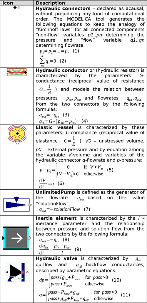
Table 1. Selected components from Physiolibrary with description
The second approach, lumped parameter approach, uses a high degree of simplification and different complex regions are generalized as single compartments characterized by lumped parameter. Using this approach, the cardiovascular system is modeled as an analogy of an electrical circuit with a set of resistors, capacitors (elastic vessels), diodes (valves) and inductance (inertial elements) in a closed loop. The relationship between pressure and volume quantities is studied throughout the modeled system. This type of model is used for the improvement of reliability in patient-specific diagnosis, for example [1,2]; or for educational purposes and training [3–9]. Technology used for modeling is either proprietary, e.g., MATLAB–Simulink or MATLAB-Simscape in the case of the CVS model introduced by Fernandez et al.[7], home grown open technology introduced by Hester et al.[3], standard grown technology from the scientific community, such as SBML[10], JSIM[11] or CellML [1,12] or industrial standard technology implemented by several vendors, such as the Modelica language [8,9].
This article introduces a modeling method which follows the second approach for modeling CVS as pressure-volume relations and introduces example models implemented in the Modelica language. We believe that one of the properties of the Modelica language – acausal modeling – seems to capture the modeled reality much better and allows connecting simpler models into quite complex systems of differential equations in an understandable form [4,13,14]. Additionally, we use a library for modeling physiology in Modelica – Physiolibrary – as the model diagrams based on the Physiolibrary components are self-descriptive in most cases [15,16].
Methods
Modelica is an object-oriented language, thus, in further text when we refer to components, models and systems they are classes, and the one's with concrete values of parameters are instances as is usual in standard object-oriented programming. Models (classes) can inherit behavior or can be composed from other models (classes). For the composition a special purpose class – connector – can be used to define variables of the model shared with other models.
The following models in the Modelica language are usually declared by an icon and defined either in diagram view or textual notation. The icon declares an interface of how the particular model instance can appear in other higher level model diagrams. The diagram and textual view declares the internal structure, which are in fact algebraic and differential equations among model parameters and variables.
As was mentioned earlier, Modelica models can be acausal, the equations can be expressed declaratively and the Modelica tool will decide which variables are dependent and independent based on the context upon compilation. This is extremely useful when several existing components are composed into a larger system model and the complexity is kept in a maintainable set of diagrams.
In further examples we use the following components from Physiolibrary (Table 1).
Two connected balloons
The model diagram (Figure 1) expresses the situation of two elastic balloons filled with liquid connected via an inelastic tube with characteristic resistance. Such a model diagram connects the system of equations of the two elastic vessels and one resistor and Modelica will figure out which variables will be independent and which will be dependent. In this example the pressure will be computed first from the initial volume of the two balloons by equation (5). This determines the pressure gradient, which directs the flow from the first balloon to the second one in equation (4). The flowrate affects the volume change in each elastic vessel in equation (6) and again causes the change of pressure from equation (5).
Windkessel models
The Windkessel models simplify the view on CVS as a series of compartments with capacity (compliance or elasticity of an elastic compartment), resistance (conductance or resistance of a conductor/resistor), impedance and inertance properties. They study the Windkessel effect, which maintains a relatively stable flowrate from the system, although the pulsatile flowrate comes from the pump. Several derivatives and improvements of Windkessel models were introduced [17].
Figures 3, 4, and 5 show diagrams of the Windkessel model of 2 elements, 3 elements and 4 elements in Modelica using Physiolibrary components. Additionally, the model diagrams contain component “pulses” declared by the icon in Figure 2 and defined by following Modelica listing:
 via a conductor (resistor).")
Figure 1. Two balloon example model diagram. It connects two balloons characterized with compliance (elastance) via a conductor (resistor).

Figure 2. Icon of component "pulses"
 C=1.4 ml/mmHg) and resistance with conductance G=1.08 ml/(mmHg.s)")
Figure 3. 2-element Windkessel model characterized by compliance component (arteries) C=1.4 ml/mmHg) and resistance with conductance G=1.08 ml/(mmHg.s)
), compliance component (arteries) C=1.4 ml/mmHg) and resistance with conductance G=1.08 ml/(mmHg.s)")
Figure 4. 3-element Windkessel model characterized by impedance (here approximated by conductance = 200ml/(mmHg.s)), compliance component (arteries) C=1.4 ml/mmHg) and resistance with conductance G=1.08 ml/(mmHg.s)
), inertia I=0.005 mmHg.s^2/ml, compliance component (arteries) C=1.4 ml/mmHg) and resistance with conductance G=1.08 ml/(mmHg.s)")
Figure 5. 4-element Windkessel model characterized by impedance (here approximate by conductance = 200ml/(mmHg.s)), inertia I=0.005 mmHg.s^2/ml, compliance component (arteries) C=1.4 ml/mmHg) and resistance with conductance G=1.08 ml/(mmHg.s)

Figure 6. Non-pulsatile circulation model diagram. Pulmonary circulation on top of the diagram is connected via side of the heart with systemic circulation at the bottom of the diagram.

Figure 7. Pulsatile heart pump model
![Figure 8. Reference model by Fernandez de Canete et al. [7] in Modelica using Physiolibrary components](/res/image/vol2-iss2/04140914-fig08.jpg "Figure 8. Reference model by Fernandez de Canete et al. [7] in Modelica using Physiolibrary components")
Figure 8. Reference model by Fernandez de Canete et al. [7] in Modelica using Physiolibrary components
. After five seconds the system is almost at equilibrium.")
Figure 9. Simulation of volume dynamics from 500 ml to 1500 ml for the first balloon and from 2000 ml to 1000 ml for the second balloon. Unstressed volumes of 500 ml for both balloons and compliances of 2 ml/mmHg and 1 ml/mmHg and conductance 1 ml/(mmHg.s). After five seconds the system is almost at equilibrium.
), inertia I=0.005 mmHg.s^2/ml, compliance component (arteries) C=1.4 ml/mmHg) and resistance with conductance G=1.08 ml/(mmHg.s) and initial volume of arteries at 0.97 l and unstressed volume of arteries at 0.85 l. The pressure during six beats is kept between 120/80 and the flowrate going from the heart ranging from 0 to 25 l per minute (blue) is compensated by the compliance compartment flowrate going from -5 to +18 l per minute (red) to the resulting average flowrate going from peripheral arteries 5 to 7 l per minute (green).")
Figure 10. Simulation of 4-element Windkessel model characterized by impedance (approximate by conductance = 200 ml/(mmHg.s)), inertia I=0.005 mmHg.s^2/ml, compliance component (arteries) C=1.4 ml/mmHg) and resistance with conductance G=1.08 ml/(mmHg.s) and initial volume of arteries at 0.97 l and unstressed volume of arteries at 0.85 l. The pressure during six beats is kept between 120/80 and the flowrate going from the heart ranging from 0 to 25 l per minute (blue) is compensated by the compliance compartment flowrate going from -5 to +18 l per minute (red) to the resulting average flowrate going from peripheral arteries 5 to 7 l per minute (green).
 and pulsatile CVS models (red)")
Figure 11. Pressure dynamics in systemic and pulmonary arteries simulated by both non-pulsatile (red) and pulsatile CVS models (red)
![Figure 12. Pressure dynamics in systemic and pulmonary artery simulated in reference model by Fernandez de Canete et al [7]](/res/image/vol2-iss2/04140914-fig12.jpg "Figure 12. Pressure dynamics in systemic and pulmonary artery simulated in reference model by Fernandez de Canete et al [7]")
Figure 12. Pressure dynamics in systemic and pulmonary artery simulated in reference model by Fernandez de Canete et al [7]
![Figure 13. Pressure dynamics in aorta (blue) and left ventricle (red) simulated in reference model by Fernandez de Canete et al. [7]. At time 0.07s the aortic valve opens and the pressure in left ventricle is only slightly higher than in aorta allowing the blood to flow from left ventricle to aorta.](/res/image/vol2-iss2/04140914-fig13.jpg "Figure 13. Pressure dynamics in aorta (blue) and left ventricle (red) simulated in reference model by Fernandez de Canete et al. [7]. At time 0.07s the aortic valve opens and the pressure in left ventricle is only slightly higher than in aorta allowing the blood to flow from left ventricle to aorta.")
Figure 13. Pressure dynamics in aorta (blue) and left ventricle (red) simulated in reference model by Fernandez de Canete et al. [7]. At time 0.07s the aortic valve opens and the pressure in left ventricle is only slightly higher than in aorta allowing the blood to flow from left ventricle to aorta.
![Figure 14. Comparison of pressure dynamics in systemic arteries simulated by simple pulsatile CVS models (blue) and by reference Fernandez de Canete model[7] implemented in Modelica (red dashed)](/res/image/vol2-iss2/04140914-fig14.jpg "Figure 14. Comparison of pressure dynamics in systemic arteries simulated by simple pulsatile CVS models (blue) and by reference Fernandez de Canete model[7] implemented in Modelica (red dashed)")
Figure 14. Comparison of pressure dynamics in systemic arteries simulated by simple pulsatile CVS models (blue) and by reference Fernandez de Canete model[7] implemented in Modelica (red dashed)
model pulses
import Physiolibrary.Types.*;
Physiolibrary.Types.RealIO.VolumeFlowRateOutput volumeflowrate;
discrete Time T0 "beginning of cardiac cycle";
Boolean b(start=false);
discrete Time HP "duration of cardiac cycle";
parameter Frequency HR = 1.2;
Time tc "relative time in cardiac cycle";
parameter Time TD1=0.07 "relative time of start of systole";
discrete Time TD2 "relative time of end of systole";
parameter VolumeFlowRate QP = 0.000424 "peak volume flowrate";
equation
b = time - pre(T0) >=pre(HP) "true if new cardiac cycle begins";
when {initial(),b} then
T0 = time "set beginning of cardiac cycle";
HP=1/HR "update length of cardiac cycle";
TD2 = TD1+(2/5)*HP "compute end time of systole";
end when;
tc = time-T0 "relative time in cardiac cycle";
volumeflowrate =
if tc<TD1 then 0 else
if tc<TD2 then sin((tc-TD1)/(TD2-TD1)*Modelica.Constants.pi)*QP else
0 "zero before and after systole, otherwise sin up to peak flow";
end pulses;
This component generates regular pulses of flowrate during the systole period, which are approximated by the sinus function increasing from zero up to the peak flowrate and back to zero during 2/5 of a cardiac cycle, while at other times it generates a zero signal. The keyword “discrete” notes the Modelica tool, wherein such variables will be changed only in discrete events, in our case at the beginning of the cardiac cycle.
A simple model of the cardiovascular system
We divide the CVS system into systemic circulation and pulmonary circulation; each circulation is characterized by a modified 2-element Windkessel model with an additional compliance component expressing the systemic and pulmonary veins (Figure 6).
The “rightHeart” and “leftHeart” components are instances of the model “HeartPump”. The flowrate of the model “HeartPump” is determined by the filling pressure and by the slope of the Starling curve. The equations are defined in the following Modelica text notation:
model HeartPump
Physiolibrary.Hydraulic.Interfaces.HydraulicPort_a inflow "inflow";
Physiolibrary.Hydraulic.Interfaces.HydraulicPort_b outflow "outflow";
parameter Physiolibrary.Types.HydraulicConductance StarlingSlope;
equation
inflow.q + outflow.q =0;
inflow.q = StarlingSlope * inflow.pressure;
end HeartPump;
The non-pulsatile model shows the mean values of pressure and flow throughout CVS. To enhance the above mentioned model, we first define the pulsatile model PulsatileHeartPump by diagram (Figure 7).
We utilize the object-oriented features in Modelica to extend the non-pulsatile circulation by only replacing the heartPump instances by pulsatile heart pump instances as seen in the following listing. Note the redefinition of values (in SI units) of parameter QP, k, volume_start:
model PulsatileCirculation
extends NonPulsatileCirculation(
redeclare Parts.PulsatileHeartPump rightHeart(pulses(QP = 0.000338)),
redeclare Parts.PulsatileHeartPump leftHeart(pulses(QP=0.000338)),
CAS(k=7.2755972857029e-09),
SystemicArteries(volume_start=0.000603),
SystemicVeins(volume_start=0.003991));
end PulsatileCirculation;
Reference model with ventricles
For further comparison purposes, we have chosen model of CVS published by Fernandez de Canete et al. implemented originally in MATLAB-Simscape [7]. This model is presented in Modelica using Physiolibrary components in one diagram (Figure 8). Systemic and pulmonary circulation are presented as modified Windkessel model with inertia element connected via heart subsystem. Additionally, each side of heart is composed by two valves and a ventricle. The ventricle is modeled as an elastic compartment driven by variable elasticity generator defined by the following Modelica listing:
model TimeVaryingElastance
parameter Physiolibrary.Types.HydraulicElastance Ed "e. of diastole";
parameter Physiolibrary.Types.HydraulicElastance Es "e.of systole";
parameter Physiolibrary.Types.Pressure Pi0 "peak isovolumic pressure";
Physiolibrary.Types.Time tm
"relative time from the beginning of cardiac cycle";
discrete Physiolibrary.Types.Time HP "heart period";
discrete Physiolibrary.Types.Time t0 "start time of the cardiac cycle";
discrete Physiolibrary.Types.Time ts "duration of systole";
Real a;
Physiolibrary.Types.RealIO.HydraulicComplianceOutput C;
Physiolibrary.Types.HydraulicElastance E;
Physiolibrary.Types.RealIO.PressureOutput Pi;
Physiolibrary.Types.RealIO.FrequencyInput HR "heart rate";
equation
tm = time - pre(t0);
if (tm<pre(ts)) then
a= (1-cos(2*Modelica.Constants.pi*tm/pre(ts)))/2;
else
a=0;
end if;
E=Ed+Es*a;
C=1/E;
Pi = Pi0*a;
when {initial(), tm >= pre(HP)} then
HP = 1/HR;
t0= time;
ts = 0.16+0.3*HP;
end when;
end TimeVaryingElastance;
Results
The two balloons model (Figure 1) is used in simulators to demonstrate that a liquid (e.g., blood) flows from the part with higher pressure to the part with lower pressure. If there is no other active force, the system converges to an equilibrium, where the pressures will be equal and no other flow occurs between the balloons (Figure 9).
This model and simulation is used to demonstrate that the blood has a tendency to flow from the arteries with lower compliance and higher pressure to the veins. Without any external force, the majority of blood accumulates in veins rather than in arteries.
Simulation of the Windkessel models imitate the heart pulses by the generator controlled with the “pulses” component (Figure 10).
The simulation of Windkessel model shows the Windkessel effect, which reduces a high variation of flowrate coming from the heart to a relatively stable flowrate in the systemic peripheral vessels due to the compliance of the elastic compartment.
The simulation of newly introduced extended model with pulsatile circulation (Figure 11) shows approximate dynamic pressure in aorta and pulmonary artery compared to the same variables of non-pulsatile model showing rather a mean values. The values of parameters and initial values of state variables are in Table 2 and 3 using normal physiological units as well as SI units.
The simulation of reference model by Fernandez de Canete et al. (Figure 8) was performed using original values of parameters (Table 4). The pressure dynamics in aorta and pulmonary arteries (Figure 12) shows quite realistic dicrotic notch after closure of aortic valve. Detailed pressure dynamics of aorta and left ventricle during one cardiac cycle is in Figure 13.
Table 2. Initial values of state variables and parameters of the non-pulsatile model of CVS in Modelica. Asterisk indicates initial volume of a component computed from steady state simulation.
|
Parameter |
Value |
Value in SI |
Ref. |
|
V0CAS.k (unstressed volume of systemic arteries) |
529 ml |
5.29x10⁻⁴ m3 |
|
|
CAS.k (compliance of systemic arteries) |
1.5 ml/mmHg |
1.13x10⁻⁸ m3/Pa |
|
|
systemicArteries.volume_start |
672 ml |
6.72x10⁻⁴ m3 |
* |
|
V0VS.k (unstressed volume of systemic veins) |
2845 ml |
2.845x10⁻³ m3 |
|
|
CVS.k (compliance of systemic veins) |
200 ml/mmHg |
1.50x10⁻⁶ m3/Pa |
|
|
systemicVeins.volume_start |
3922 ml |
3.922x10⁻³ m3 |
* |
|
V0AP.k (unstressed volume of pulmonary arteries) |
327 ml |
3.27x10⁻⁴ m3 |
|
|
CAP.k (compliance of pulmonary arteries) |
3.01 ml/mmHg |
2.26x10⁻⁸ m3/Pa |
|
|
pulmonaryArteries.volume_start |
373 ml |
3.73x10⁻⁴ m3 |
* |
|
V0VP.k (unstressed volume of pulmonary veins) |
435 ml |
4.35x10⁻⁴ m3 |
|
|
CVP.k (compliance of pulmonary veins) |
30 ml/mmHg |
2.25x10⁻⁷ m3/Pa |
|
|
pulmonaryVeins.volume_start |
704 ml |
7.04x10⁻⁴ m3 |
* |
|
RT.k (total systemic resistance) |
1 (mmHg.s)/ml |
1.33x10⁸ (Pa.s)/m3 |
|
|
RP.k (total pulmonary resistance) |
0.07 (mmHg.s)/ml |
9.33x10⁶ (Pa.s)/m3 |
|
|
rightHeart.StarlingSlope |
16.67 ml/(mmHg.s) |
1.25x10⁻⁷ m3/(Pa.s) |
|
|
leftHeart.StarlingSlope |
10 ml/(mmHg.s) |
7.50x10⁻⁸ m3/(Pa.s) |
|
Table 3. Additional initial values of state variables and parameters of the pulsatile model of CVS in Modelica. Decreased value of CAS and changed initial volumes of systemic arteries and veins to compare with reference model. Other values inherited from non-pulsatile model (Table 2).
|
Parameter |
Value |
Value in SI |
Ref. |
|
CAS.k (compliance of systemic arteries) |
0.97 ml/mmHg |
7.28x10⁻⁹ m3/Pa |
|
|
systemicArteries.volume_start |
603 ml |
6.03x10⁻⁴ m3 |
* |
|
systemicVeins.volume_start |
3991 ml |
3.991x10⁻³ m3 |
* |
|
rightHeart.pulses.QP (peak flow of right heart) |
20.28 l/min |
3.38x10⁻⁴ m3/s |
|
|
leftHeart.pulses.QP (peak flow of left heart) |
20.28 l/min |
3.38x10⁻⁴ m3/s |
|
|
pulses.HR (default heart rate) |
72 beats per min |
1.2 Hz |
|
|
Pulses.TD1 (relative time of systole start) |
0.07 s |
0.07 s |
|
Table 4. Initial values of state variables and parameters of the reference model by Fernandez de Canete et al. [7] in Modelica. Values with reference were taken from the original publication, asterisk indicates initial values computed from steady state simulation, other values were estimated. “ZeroPressureVolume” is unstressed volume of a component, “volume_start” is initial volume of a component. “_Gon” is conductance of a valve in opened state. Compliance and conductance values were counted as reciprocal (1/x) of original elastance and resistance values.
|
Parameter |
Value |
Value in SI |
Ref. |
|
aorta.ZeroPressureVolume |
30 ml |
3.00x10⁻⁵ m3 |
|
|
aorta.Compliance |
0.22 ml/mmHg |
1.65x10⁻⁹ m3/Pa |
[7] |
|
aorta.volume_start |
46 ml |
4.60x10⁻⁵ m3 |
* |
|
arteries.ZeroPressureVolume |
700 ml |
7.00x10⁻⁴ m3 |
|
|
arteries.Compliance |
1.46 ml/mmHg |
1.10x10⁻⁸ m3/Pa |
[7] |
|
arteries.volume_start |
805 ml |
8.05x10⁻⁴ m3 |
* |
|
veins.ZeroPressureVolume |
2370 ml |
2.37x10⁻³ m3 |
|
|
veins.Compliance |
20 ml/mmHg |
1.50x10⁻⁷ m3/Pa |
[7] |
|
veins.volume_start |
2443 ml |
2.44x10⁻³ m3 |
* |
|
pulmonaryArtery.ZeroPressureVolume |
20 ml |
2.00x10⁻⁵ m3 |
|
|
pulmonaryArtery.Compliance |
0.09 ml/mmHg |
6.75x10⁻¹⁰ m3/Pa |
[7] |
|
pulmonaryArtery.volume_start |
21 ml |
2.10x10⁻⁵ m3 |
* |
|
pulmonaryArterioles.ZeroPressureVolume |
600 ml |
6.00x10⁻⁴ m3 |
|
|
pulmonaryArterioles.Compliance |
2.67 ml/mmHg |
2.00x10⁻⁸ m3/Pa |
[7] |
|
pulmonaryArterioles.volume_start |
637 ml |
6.37x10⁻⁴ m3 |
* |
|
pulmonaryVeins.ZeroPressureVolume |
100 ml |
1.00x10⁻⁴ m3 |
|
|
pulmonaryVeins.Compliance |
46.7 ml/mmHg |
3.50x10⁻⁷ m3/Pa |
[7] |
|
pulmonaryVeins.volume_start |
659.7 ml |
6.597x10⁻⁴ m3 |
* |
|
heartRate.k |
72 1/min |
1.2 Hz |
|
|
leftVentricle.ZeroPressureVolume |
90 ml |
9.00x10⁻⁵ m3 |
|
|
leftVentricle.volume_start |
209.7 ml |
2.097x10⁻⁴ m3 |
* |
|
timeVaryingElastanceLeft.Ed |
0.1 mmHg/ml |
1.33x10⁷ Pa/m3 |
[7] |
|
timeVaryingElastanceLeft.Es |
1.375 mmHg/ml |
1.83x10⁸ Pa/m3 |
[7] |
|
timeVaryingElastanceLeft.Pi0 |
50 mmHg |
6.66x10³ Pa |
[7] |
|
rightVentricle.ZeroPressureVolume |
70 ml |
7.00x10⁻⁵ m3 |
|
|
rightVentricle.volume_start |
180 ml |
1.80x10⁻⁴ m3 |
|
|
timeVaryingElastanceRight.Ed |
0.03 mmHg/ml |
4.00x10⁶ Pa/m3 |
[7] |
|
timeVaryingElastanceRight.Es |
0.328 mmHg/ml |
4.37x10⁷ Pa/m3 |
[7] |
|
timeVaryingElastanceRight.Pi0 |
24 mmHg |
3.20x10³ Pa |
[7] |
|
mitralValve._Gon |
266.6 ml/(mmHg.s) |
2.00x10⁻⁶ m3/(Pa.s) |
[7] |
|
RleftMyo.Conductance |
12.5 ml/(mmHg.s) |
9.37x10⁻⁸ m3/(Pa.s) |
[7] |
|
aorticValve._Gon |
266.6 ml/(mmHg.s) |
2.00x10⁻⁶ m3/(Pa.s) |
[7] |
|
Raorta.Conductance |
14.81 ml/(mmHg.s) |
1.11x10⁻⁷ m3/(Pa.s) |
[7] |
|
Rsystemic.Conductance |
1 ml/(mmHg.s) |
7.50x10⁻⁹ m3/(Pa.s) |
[7] |
|
tricuspidValve._Gon |
266.6 ml/(mmHg.s) |
2.00x10⁻⁶ m3/(Pa.s) |
[7] |
|
RRightMyo.Conductance |
57.14 ml/(mmHg.s) |
4.29x10⁻⁷ m3/(Pa.s) |
[7] |
|
pulmonaryValve._Gon |
266.6 ml/(mmHg.s) |
2.00x10⁻⁶ m3/(Pa.s) |
[7] |
|
RPulmonaryArtery.Conductance |
29.62 ml/(mmHg.s) |
2.22x10⁻⁷ m3/(Pa.s) |
[7] |
|
RPulmonaryVeins.Conductance |
9.9 ml/(mmHg.s) |
7.43x10⁻⁸ m3/(Pa.s) |
[7] |
|
aorticInertia.I |
8.25x10⁻⁴ mmHg.s2/ml |
1.10x10⁵ Pa.s2/m3 |
[7] |
|
aorticInertia.volumeFlow_start |
623.1 ml/min |
1.04x10⁻⁵ m3/s |
* |
|
systemicInertia.I |
3.6x10⁻³ mmHg.s2/ml |
4.80x10⁵ Pa.s2/m3 |
[7] |
|
systemicInertia.volumeFlow_start |
4761 ml/min |
7.94x10⁻⁵ m3/s |
* |
|
pulmonaryArterialInertia.I |
7.5x10⁻⁴ mmHg.s2/ml |
1.00x10⁵ Pa.s2/m3 |
[7] |
|
pulmonaryArterialInertia.volumeFlow_start |
43.94 ml/min |
7.32x10⁻⁷ m3/s |
* |
|
pulmonaryVeinsInertia.I |
3.08x10⁻³ mmHg.s2/ml |
4.11x10⁵ Pa.s2/m3 |
[7] |
|
pulmonaryVeinsInertia.volumeFlow_start |
1335 ml/min |
2.23x10⁻⁵ m3/s |
* |
Discussion
Our non-pulsatile and pulsatile models generate a raw approximation of outgoing flowrate. However, other models, such as the model developed by Fernandez de Cante et al. [7,8], or that developed by Meurs et al. [5,6], introduce a heart with elastic vessels driven by variable compliance and valves rather than a pump with variable outgoing flowrate. The shapes of the pressure curves in these models are closer to the real experimental measurements.
In order to study more specific phenomena, additional components can be added to the model. For instance, our implementation does not use the inertia element and valves. This seems to be useful for examining the effect of a dicrotic notch in the arterial pressure when the aortic valve closes as seen, for instance, in the model and simulation developed by Fernandez de Canete et al. [7]. Figure 14 shows comparison with simple pulsatile model.
Our implementation uses one resistance and two elastic vessel components for the pulmonary and systemic circulation with total of 16 parameters and initial values of state variables (Table 2). The pulsatile model adds new 4 parameters and redefine values of three existing (Table 4). This seems satisfactory to explain basic physiological and pathophysiological phenomena, e.g. influence of congestive left or right heart failure to volumes of blood in systemic or pulmonary veins. The more realistic models with additional components introduce also additional parameters and initial values for state variables. The CVS model by Fernandez de Canete et al. [7] has 48 parameters (Table 4) and this may cause some confusion when teaching only the effects described above. But these more complex models are, however, more suitable to study e.g. the phases within cardiac cycle as seen in Figure 12.
The non-pulsatile model (Figure 6) is a base of an existing educational application simple circulation available in the Atlas of Physiology and Pathophysiology (www.physiome.cz/atlas) [18] and is used in teaching physiology and pathophysiology of cardiovascular system of students of medicine and biomedical engineering[19,20]. The new pulsatile model is used in further development of the simulators to describe additionally the Windkessel effect. The simulators are introduced in lectures of pathophysiology for students of medicine and several basic scenarios are demonstrated. Students, according to surveys, use the simulators again at home when they prepare for tests and exams. This has been acknowledged as an improvement of understanding complex relation and mechanism in CVS compared to static text or non-interactive e-learning materials.
The models introduced above are used in teaching modeling and simulation of students of biomedical engineering. Because the physical system can be decomposed into basic components and modeled in an understandable form, the students focus much more on system analysis rather than on implementation issues [21].
There are some general limitations to the models based on the Windkessel phenomenon and modeling pressure volume relationship, e.g., wave transmission and wave travel cannot be studied.
Conclusion
Modeling technique and example models were introduced to demonstrate some effects that are important in understanding the physiology of the cardiovascular system, e.g. flow is determined by pressure gradient and Windkessel effect stabilizes the flowrate changes going from the heart to the peripheral vessels.
The implementation in Modelica language, utilizing the open source Physiolibrary, allows the expression of a complex system of differential and algebraic equations in self-descriptive model diagrams. The mathematics is hidden in the low level component model definition.
The newly introduced pulsatile model of CVS is used in further development of educational simulators.
A full source code of presented models is attached as supplementary materials to this paper and can be tried in the commercial tool Dymola or in the open source tool OpenModelica (www.openmodelica.org) using Physiolibrary (www.physiolibrary.org).
Acknowledgments
This paper describes the outcome of research that has been accomplished as part of a research program funded by the Ministry of Industry and Trade of the Czech Republic via grant FR-TI3/869; and by the Ministry of Education, Youth and Sports via the grant SVV-2014-260033.
References
1. Smith BW, Chase JG, Nokes RI, Shaw GM, Wake G. Minimal Haemodynamic System Model Including Ventricular Interaction and Valve Dynamics. Med Eng Phys 2004; 26(2): 131-139.
2. Revie JA, Stevenson DJ, Chase JG, Hann CE, Lambermont BC, Ghuysen A, Kolh P, Shaw GM, Heldmann S, Desaive T. Validation of Subject-Specific Cardiovascular System Models from Porcine Measurements. Comput Methods Programs Biomed 2013; 109(2): 197-210.
3. Hester RL, Brown AJ, Husband L, Iliescu R, Pruett D, Summers R, Coleman TG. HumMod: A Modeling Environment for the Simulation of Integrative Human Physiology. Front Physiol 2011; 2: 12.
4. Kofránek J, Mateják M, Privitzer P. Complex Model of Integrated Physiological System - A Theoretical Basis For Medical Training Simulators. Mefanet Report 04 2011: 32-59.
5. Van Meurs W. Modeling and Simulation in Biomedical Engineering: Applications in Cardiorespiratory Physiology. McGraw-Hill Professional 2011.
6. Sá Couto CD, van Meurs WL, Goodwin JA, Andriessen P. A Model for Educational Simulation of Neonatal Cardiovascular Pathophysiology. Simul Healthc 2006; 1(1): 4-12.
7. Fernandez de Canete J, del Saz-Orozco P, Moreno-Boza D, Duran-Venegas E. Object-Oriented Modeling and Simulation of the Closed Loop Cardiovascular System by Using SIMSCAPE. Comput Biol Med 2013; 43(4): 323-33.
8. Fernandez de Canete J, Luque J, Barbancho J, Munoz V. Modelling of Long-Term and Short-Term Mechanisms of Arterial Pressure Control in the Cardiovascular System: An Object-Oriented Approach. Comput Biol Med 2014; 47: 104-112.
9. Kofránek J. Modelica. In: Sborník Příspěvků MEDSOFT. 2013; 64-114.
10. Hucka M, Finney A, Bornstein BJ, Keating SM, Shapiro BE, Matthews J, Kovitz BL, Schilstra MJ, Funahashi A, Doyle JC. Evolving a Lingua Franca and Associated Software Infrastructure for Computational Systems Biology: The Systems Biology Markup Language (SBML) Project. Syst Biol (Stevenage) 2004; 1(1): 41-53.
11. Butterworth E, Jardine BE, Raymond GM, Neal ML, Bassingthwaighte JB. JSim, an Open-Source Modeling System for Data Analysis. F1000Research 2014; 2: 288.
12. Cooling M, Hunter P, Crampin E. Modelling Biological Modularity with CellML. IET Syst Biol 2008; 2(2): 73-79.
13. Kofránek J, Mateják M, Privitzer P, Tribula M. Causal or Acausal Modeling: Labour for Humans or Labour for Machines. Tech Comput Prague 2008: 1-16.
14. Kulhánek T, Kofránek J, Mateják M. Modeling of Short-Term Mechanism of Arterial Pressure Control in the Cardiovascular System: Object Oriented and Acausal Approach. Comput Biol Med 2014; 54(1): 137-144.
15. Mateják M. Physiology in Modelica. Mefanet J 2014; 2(1): 10-14.
16. Mateják M, Kulhánek T, Šilar J, Privitzer P, Ježek F, Kofránek J. Physiolibrary - Modelica Library for Physiology. In: Proc. 10th Int. Model. Conf. March 10-12, 2014, Lund, Sweden. Linköping University Electronic Press 2014: 499-505.
17. Westerhof N, Lankhaar J-W, Westerhof BE. The Arterial Windkessel. Med Biol Eng Comput 2009; 47(2): 131-141.
18. Kofranek J, Matousek S, Rusz J, Stodulka P, Privitzer P, Matejak M, Tribula M. The Atlas of Physiology and Pathophysiology: Web-Based Multimedia Enabled Interactive Simulations. Comput Methods Programs Biomed 2011; 104(2): 143-53.
19. Kofránek J, Mateják M, Ježek F, Privitzer P, Šilar J. Výukový webový simulator krevního oběhu. In: Sborník Příspěvků MEDSOFT 2011: 106-121.
20. Tribula M, Ježek F, Privitzer P, Kofránek J, Kolman J. Webový výukový simulátor krevního oběhu. In: Sborník Příspěvků MEDSOFT 2013: 197-204.
21. Ježek F, Kroček T, Mateják M, Kofránek J. Zkušenosti Z Inovace Výuky Modelování a Simulace Na FEL ČVUT. In: Sborník Příspěvků MEDSOFT 2012: 139-146.
Please cite as:
Kulhánek T, Tribula M, Kofránek J, Mateják M. Simple models of the cardiovascular system for educational and research purposes. MEFANET Journal 2014; 2(2): 56-63. Available at WWW: http://mj.mefanet.cz/mj-04140914.
This is an open-access article distributed under the terms of the Creative Commons Attribution-NonCommercial-ShareAlike 3.0 License (http://creativecommons.org/licenses/by-nc-sa/3.0/), which permits unrestricted use, distribution, and reproduction in any medium, provided the original work, first published in the MEFANET Journal, is properly cited. The complete bibliographic information, a link to the original publication on http://www.mj.mefanet.cz/, as well as this copyright and license information must be included.